Meta-learning, also known as “learning to learn”, intends to design models that can learn new skills or adapt to new environments rapidly with a few training examples. There are three common approaches: 1) learn an efficient distance metric (metric-based); 2) use (recurrent) network with external or internal memory (model-based); 3) optimize the model parameters explicitly for fast learning (optimization-based).
Learner and Meta-Learner
Another popular view of meta-learning decomposes the model update into two stages:
- A classifier $f_{\theta}$ is the “learner” model, trained for operating a given task;
- In the meantime, a optimizer $g_{\phi}$ learns how to update the learner model’s parameters via the support set $S$, $\theta’ = g_\phi(\theta, S)$
Common Approaches to Meta-Learning
There are three common approaches to meta-learning: metric-based, model-based, and optimization-based.

Metric-Based
The core idea in metric-based meta-learning is similar to nearest neighbors algorithms (i.e., k-NN classificer and k-means clustering) and kernel density estimation. The predicted probability over a set of known labels $y$ is a weighted sum of labels of support set samples. The weight is generated by a kernel function $k_{\theta}$, measuring the similarity between two data samples.
$$P_\theta(y \vert \mathbf{x}, S) = \sum_{(\mathbf{x}_i, y_i) \in S} k_\theta(\mathbf{x}, \mathbf{x}_i)y_i$$
where $S$ is the support set.
To learn a good kernel is crucial to the success of a metric-based meta-learning model. Metric learning is well aligned with this intention, as it aims to learn a metric or distance function over objects. The notion of a good metric is problem-dependent. It should represent the relationship between inputs in the task space and facilitate problem solving.
Convolutional Siamese Neural Network
Siamese Neural Network 由两个孪生的网络组成,它们的输出通过一个相似度函数来衡量输入数据点之间的相似性,这两个孪生网络实际上是完全相同的特征提取器,然后再将提取出来的两个特征向量通过一个核函数计算关系。
Koch, Zemel & Salakhutdinov (2015) 提出了基于Siamese Neural Network的方法来解决one-shot的图像分类任务(每一类图片仅有一个标注样本)。整体结构图如下:
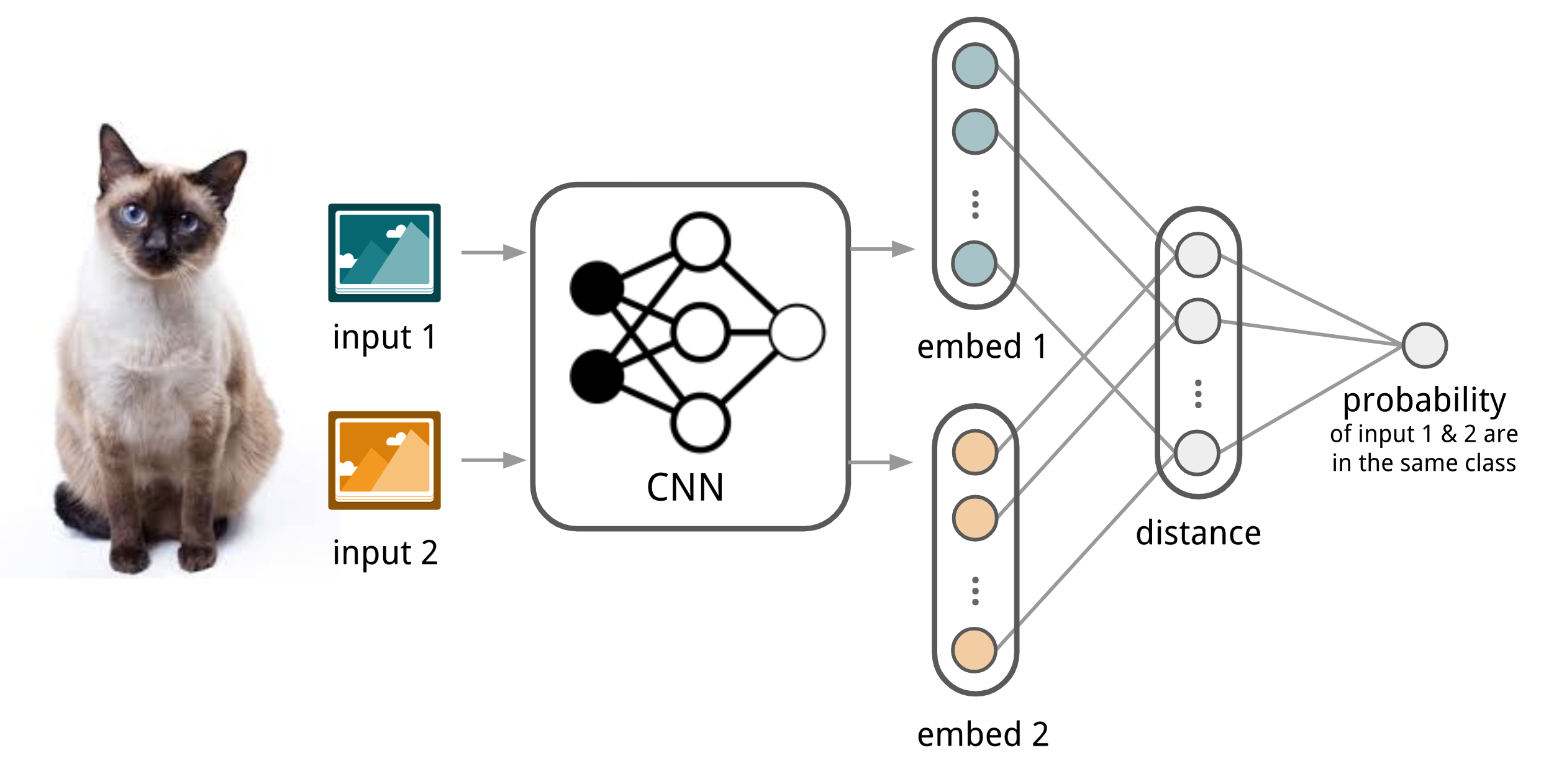
首先基于给定的$K$类数据集来构建很多二分类数据集(Support Set),然后在所有二分类数据集上训练一个鉴别模型:判断输入的两张图片是否来自同一个类别。在预测阶段,训练后的siamese network预测所有的输入图片-支持集图片对,最终的结果类别为相似度最高的支持集图片对应的类别。
Matching Networks
The task of Matching Networks (Vinyals et al., 2016) is to learn a classifier $c_{S}$ for any given (small) support set $S=\{x_{i},y_{i}\}^{k}_{i=1}$(k-class classification). This classifier defines a probability distribution over output labels $y$ given a test example $x$. Similar to other metric-based models, the classifier output is defined as a sum of labels of support samples weighted by attention kernel $a(x,x_{i})$ - which should be proportional to the similarity between $x$ and $x_{i}$.
$$c_S(\mathbf{x}) = P(y \vert \mathbf{x}, S) = \sum_{i=1}^k a(\mathbf{x}, \mathbf{x}_i) y_i
\text{, where }S=\{(\mathbf{x}_i, y_i)\}_{i=1}^k$$
The attention kernel depends on two embedding functions, $f$ and $g$, for encoding the test sample and the support set samples respectively. The attention weight between two data points is the cosine similarity, $cosine(\cdot)$, between their embedding vectors, normalized by softmax:
$$a(\mathbf{x}, \mathbf{x}_i) = \frac{\exp(\text{cosine}(f(\mathbf{x}), g(\mathbf{x}_i))}{\sum_{j=1}^k\exp(\text{cosine}(f(\mathbf{x}), g(\mathbf{x}_j))}$$
Simple Embedding In the simple version, an embedding function is a neural network with a single data sample as input. Potentially we can set $f=g$.
Full Context Embeddings The embedding vectors are critical inputs for building a good classifier. Taking a single data point as input might not be enough to efficiently gauge the entire feature space. Therefore, the Matching Network model further proposed to enhance the embedding functions by taking as input the whole support set $S$ in addition to the original input, so that the learned embedding can be adjusted based on the relationship with other support samples.
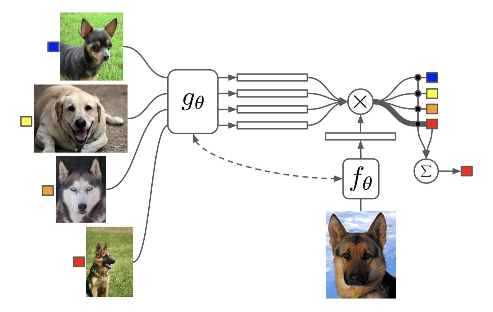
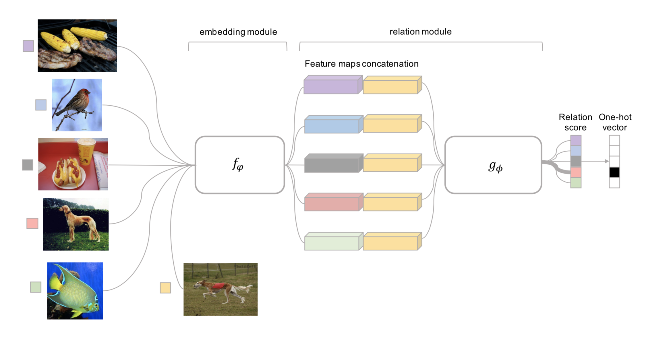
Relation Network
Relation Network (RN) (Sung et al., 2018) is similar to siamese network but with a few differences:
- The relationship is not captured by a simple L1 distance in the feature space, but predicted by a CNN classifier $g_{\phi}$. The relation score between a pair of inputs, $x_{i}$ and $x_{j}$, is $r_{ij}=g_{\phi}([x_{i},x_{j}])$ where $[]$ is concatenation.
- The objective function is MSE loss instead of cross-entropy, because conceptually RN focuses more on predicting relation scores which is more like regression, rather than binary classification. $\mathcal{L}(B) = \sum_{(\mathbf{x}_i, \mathbf{x}_j, y_i, y_j)\in B} (r_{ij} - \mathbf{1}_{y_i=y_j})^2$
Prototypical Networks
Prototypical Networks (Snell, Swersky & Zemel, 2017) use an embedding function $f_{\theta}$ to encode each input into a $M$-dimensional feature vector. A _prototype_ feature vector is defined for every class $c\in C$, as the mean vector of the embedded support data samples in this class.
$$\mathbf{v}_c = \frac{1}{|S_c|} \sum_{(\mathbf{x}_i, y_i) \in S_c} f_\theta(\mathbf{x}_i)$$
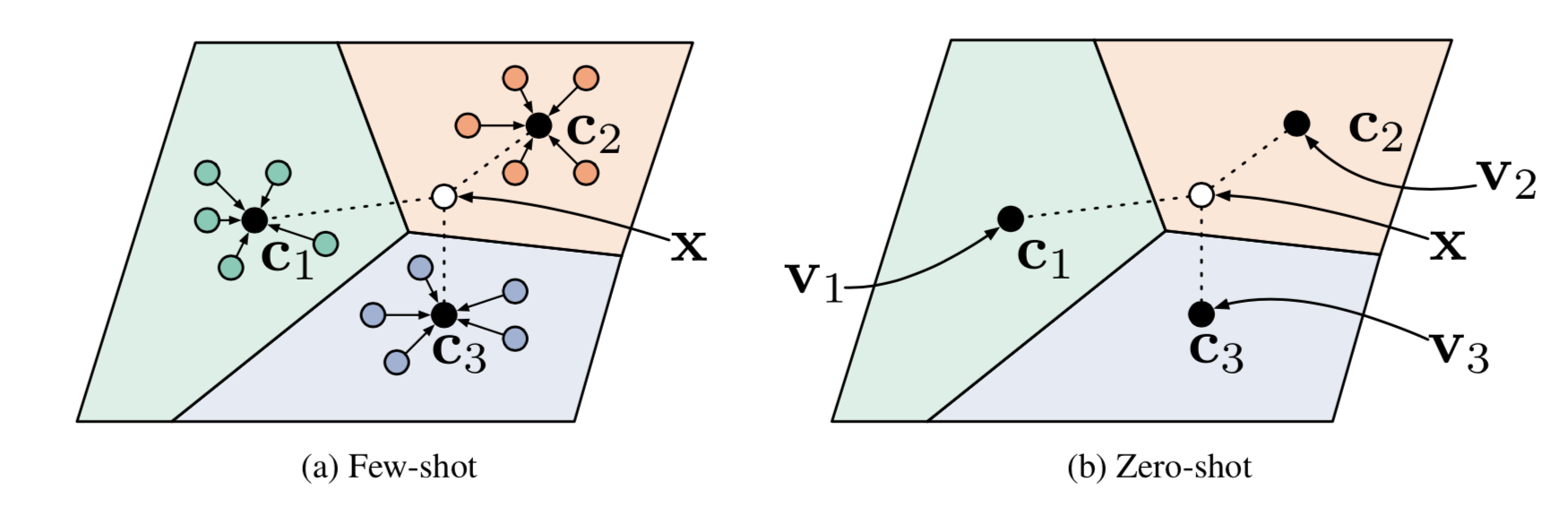
$$P(y=c\vert\mathbf{x})=\text{softmax}(-d_\varphi(f_\theta(\mathbf{x}), \mathbf{v}_c)) = \frac{\exp(-d_\varphi(f_\theta(\mathbf{x}), \mathbf{v}_c))}{\sum_{c’ \in \mathcal{C}}\exp(-d_\varphi(f_\theta(\mathbf{x}), \mathbf{v}_{c’}))}$$
where $d_\varphi$ can be any distance function as long as $\varphi$ is differentiable. In the paper, they used the squared euclidean distance. The loss function is the negative log-likelihood: $\mathcal{L}(\theta) = -\log P_\theta(y=c\vert\mathbf{x})$
Model-Based
Model-based meta-learning models make no assumption on the form of $P_{\theta}(y|x)$. Rather it depends on a model designed specifically for fast learning — a model that updates its parameters rapidly with a few training steps. This rapid parameter update can be achieved by its internal architecture or controlled by another meta-learner model.
Memory-Augmented Neural Networks
A family of model architectures use external memory storage to facilitate the learning process of neural networks, including Neural Turing Machines and Memory Networks. Such a model is known as MANN, short for “Memory-Augmented Neural Network”. Note that recurrent neural networks with only _internal memory_ such as vanilla RNN or LSTM are not MANNs.
MANN for Meta-Learning The training described in Santoro et al., 2016 happens in an interesting way so that the memory is forced to hold information for longer until the appropriate labels are presented later. In each training episode, the truth label $y_{t}$ is presented with one step offset, $(x_{t+1},y_{t})$: it is the true label for the input at the previous time step $t$, but presented as part of the input at time step $t+1$.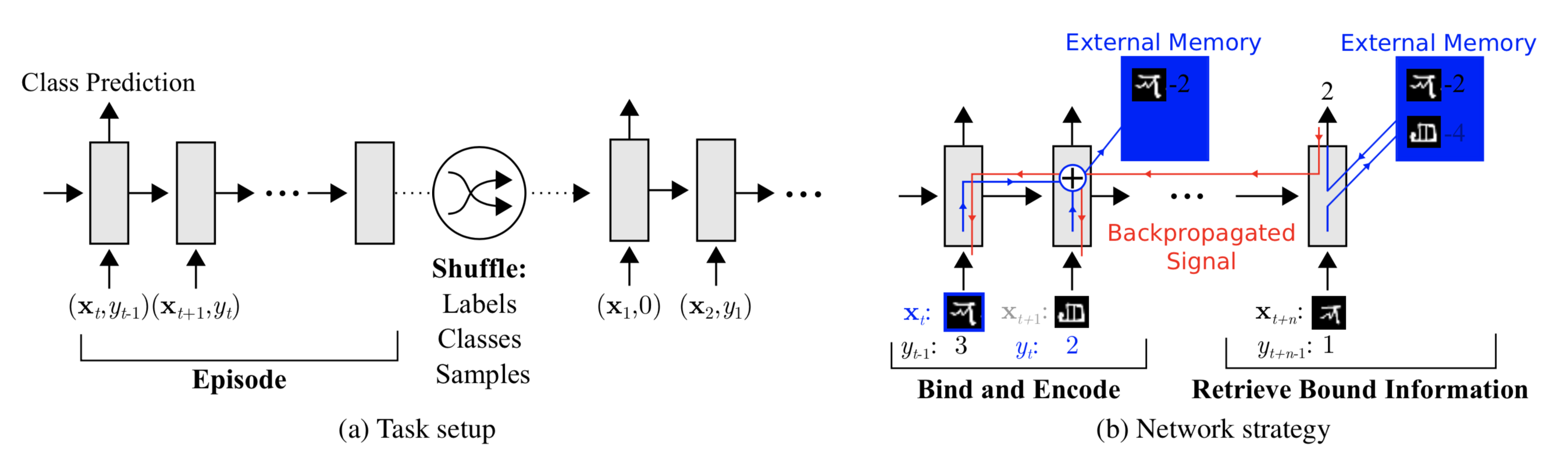
Meta Networks
Meta Networks (Munkhdalai & Yu, 2017), short for MetaNet, is a meta-learning model with architecture and training process designed for _rapid_ generalization across tasks.
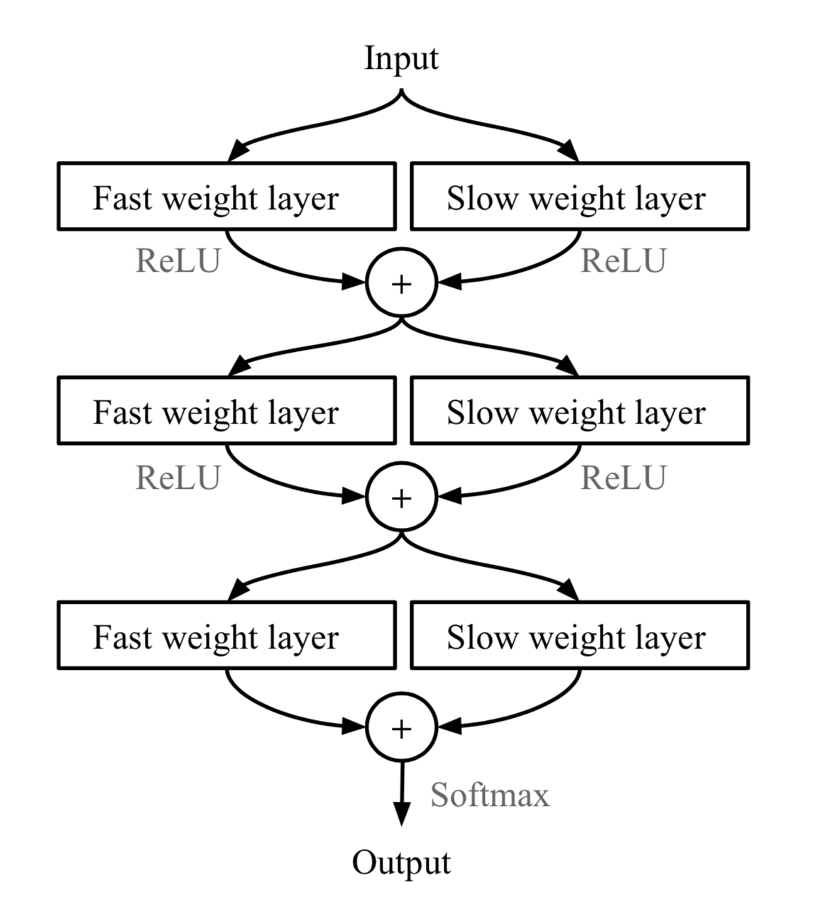
Fast Weights The rapid generalization of MetaNet relies on “fast weights”. Normally weights in the neural networks are updated by stochastic gradient descent in an objective function and this process is known to be slow. One faster way to learn is to utilize one neural network to predict the parameters of another neural network and the generated weights are called _fast weights_. In comparison, the ordinary SGD-based weights are named _slow weights_.
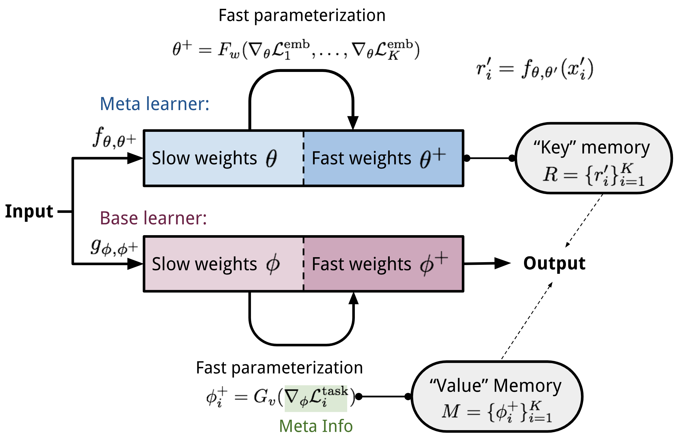
In MetaNet, loss gradients are used as _meta information_ to populate models that learn fast weights. Slow and fast weights are combined to make predictions in neural networks.
_More details in https://lilianweng.github.io/lil-log/2018/11/30/meta-learning.html#meta-networks_
Optimization-Based
Deep learning models learn through backpropagation of gradients. However, the gradient-based optimization is neither designed to cope with a small number of training samples, nor to converge within a small number of optimization steps. Is there a way to adjust the optimization algorithm so that the model can be good at learning with a few examples? This is what optimization-based approach meta-learning algorithms intend for.
LSTM Meta-Learner
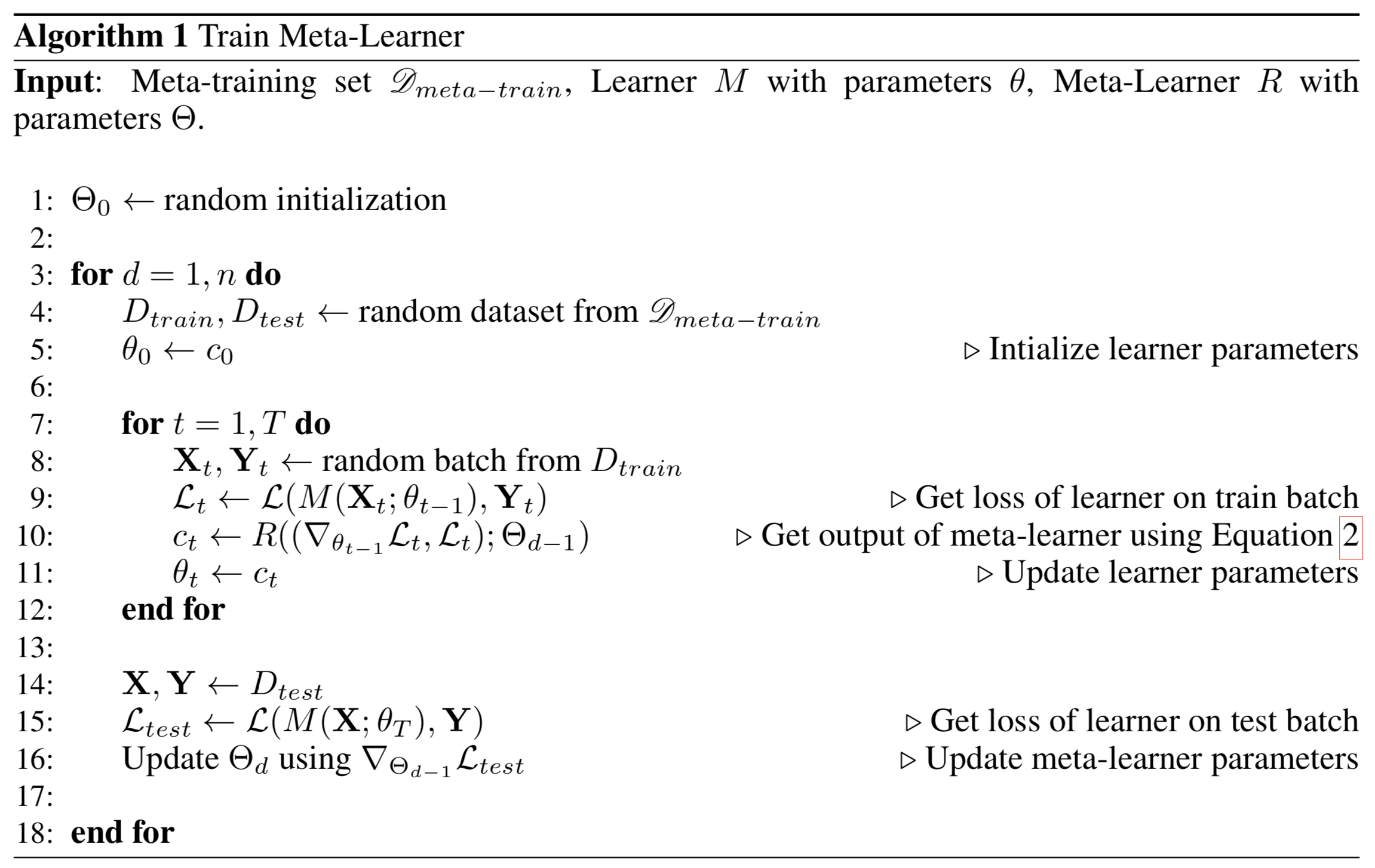
The optimization algorithm can be explicitly modeled. Ravi & Larochelle (2017) did so and named it “meta-learner”, while the original model for handling the task is called “learner”. The goal of the meta-learner is to efficiently update the learner’s parameters using a small support set so that the learner can adapt to the new task quickly.
Let’s denote the learner model as parameterized by , the meta-learner as with parameters , and the loss function. The meta-learner is modeled as a LSTM, because:
- There is similarity between the gradient-based update in backpropagation and the cell-state update in LSTM.
- Knowing a history of gradients benefits the gradient update; think about how momentum works.
The update for the learner’s parameters at time step $t$ with a learning rate $\alpha_{t}$ is:
$$\theta_t = \theta_{t-1} - \alpha_t \nabla_{\theta_{t-1}}\mathcal{L}_t$$
It has the same form as the cell state update in LSTM, if we set forget gate $f_{t}=1$, input gate $i_{t}=\alpha_{t}$, cell state $c_{t}=\theta_{t}$, and new cell state $\tilde{c}_t = -\nabla_{\theta_{t-1}}\mathcal{L}_t$:
$$c_t = f_t \odot c_{t-1} + i_t \odot \tilde{c}_t
= \theta_{t-1} - \alpha_t\nabla_{\theta_{t-1}}\mathcal{L}_t$$
While fixing $f_{t}=1$ and $i_{t}=\alpha_{t}$ might not be the optimal, both of them can be learnable and adaptable to different datasets.
Model Setup
During each training epoch, we first sample a dataset $\mathcal{D} = (\mathcal{D}_\text{train}, \mathcal{D}_\text{test}) \in \hat{\mathcal{D}}_\text{meta-train}$ and then sample mini-batches out of $D_{train}$ to update $\theta$ for $T$ rounds. The final state of the learner parameter $\theta_{T}$ is used to train the meta-learner on the test data $D_{test}$.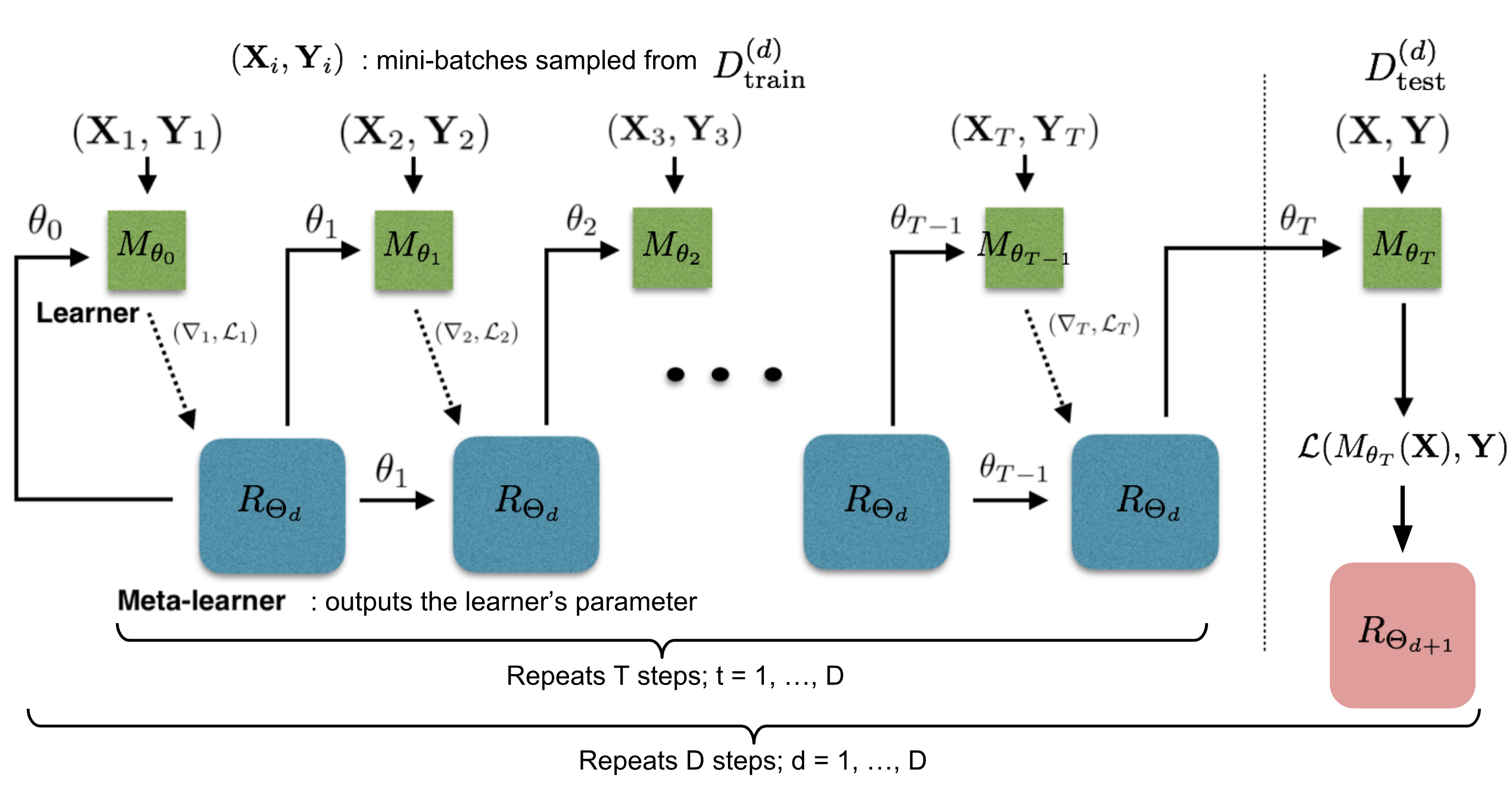
MAML
MAML, short for Model-Agnostic Meta-Learning (Finn, et al. 2017) is a fairly general optimization algorithm, compatible with any model that learns through gradient descent.
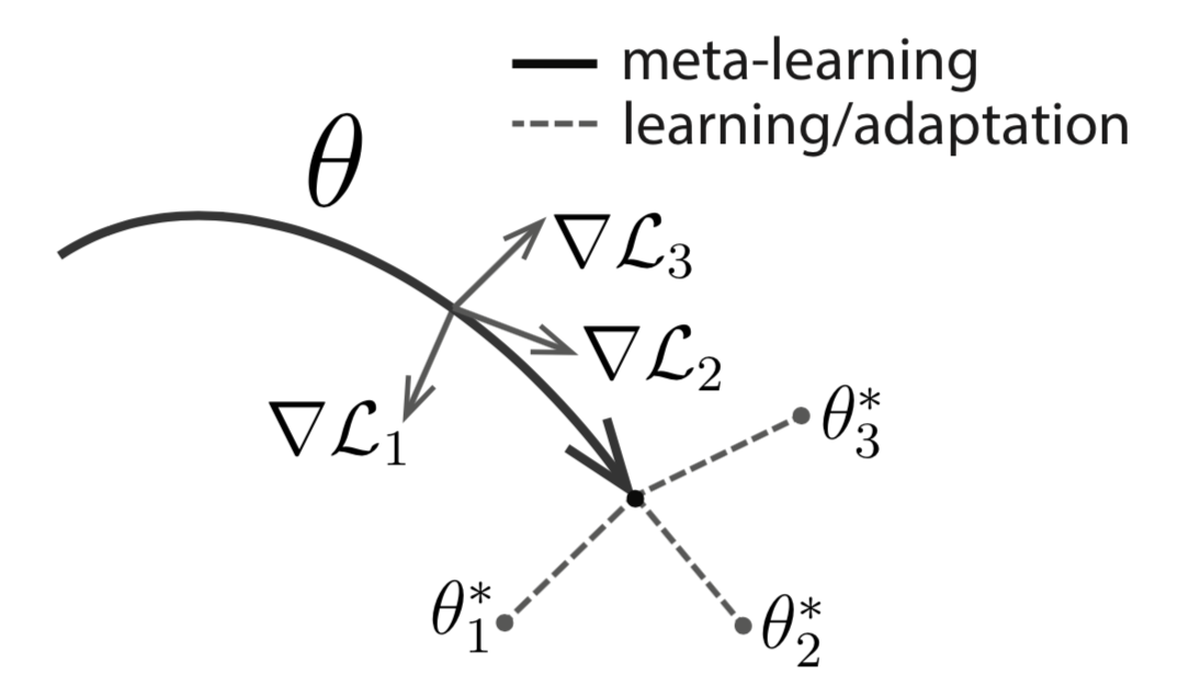
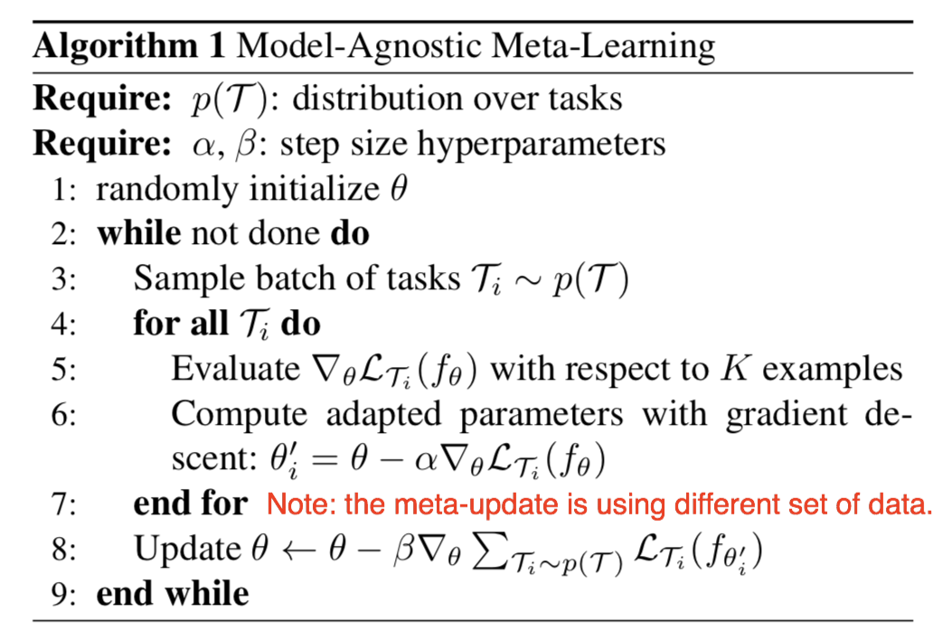
在Meta-Train阶段,更新得到 $\theta’_{i}$时,使用的是每个任务的train数据集;而在外层更新$\theta$时 ,loss函数是在test集合上的loss,对原 $\theta$(注意不是对$\theta’_{i}$)进行梯度下降。
The meta-optimization step above relies on second derivatives. To make the computation less expensive, a modified version of MAML omits second derivatives, resulting in a simplified and cheaper implementation, known as First-Order MAML (FOMAML).